|
ICORN: Iterative Correction of Reference Nucleotides |

|
Example
Here is an example of ICORN correcting parts of the chromosome one of Plasmodium falciparum strain 3D7. There will be screenshots of the different features.Motivation to see errors and their correction

Run ICORN
- It is assumed you installed ICORN and the first party software (see Manual).
- ICORN was tested in UNIX/Linux enviroments.
- Download the files MAL1.fasta, MAL1.F.fastq.gz and MAL1.R.fastq.gz in a working directory.
- Run ICORN:
$ICORN_HOME/icorn.start.sh MAL1.fasta 1 5 MAL1.F.fastq.gz MAL1.R.fastq.gz 80,250 120 76 - As this is an example, just some regions of MAL1 are chosen. Anyhow, depending the machine, your processing time should be around on nice lunch in a pub with a good pint. (A recent machine takes 40 minutes and need 1GB of memory)
If you don't want to run ICORN
Alternatively you do not want to go for lunch and drink some coffee, you can also just download the result files here.Results file
If you want to work with the corrected sequence (and you trust ICORN), you will have the corrected sequence in Reference.correct.fa. You can load the plots/MAL1.perfectmapping.plot, to see, where no reads map perfectly. Example: Screenshot of Artemis of the above shown region (with a subset of the reads).
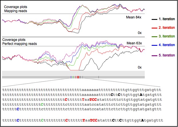
To see the figure bigger, please open it in a new window (right click). The upper graphs shows the perfect mapping reads coverage plots: red lines are before the correction, blue after the 5. iteration. Second graphs are the SSAHA coverage plots of the first five iterations. Boxes are the found errors. Gray first iteration, red second, green third. The writen annotation lines give information of the found corrections, for example the coverage of perfect mapping reads before and after the correction.
In case you want to track down the changes, please continue reading:
- Stats.Mapping.csv - shows the mapping stats. Important are the amount of uniquely mapping reads and the amount of regions in the genome covered more than 20 times. Interesting is also the amount of reads that map in each iteration. As the sequence get more and more correct, more reads can be mapped.
Example of Stats.Mapping.csv:
- Stats.Correction.csv - Show the correction of each iteration for each "correction Tag". In the first iteration most errors are found, but not all. HETERO are position where another allele is found with the ratio of 0.15.
Example of Stats.Correction.csv:
- All.MAL1.gff - File for Artemis with all the changes. One should load this file in artemis, but it can also be parsed easily in other formats, i.e. GAP4.
- plots/ - Four plots are done. Perfect mapping reads for the original version of the MAL1 sequence and of the best corrected. The same is done for the SSAHA coverage plots. Perfect mapping means, that reads that have no different to the sequence are mapped. Therefore errors can be seen when the coverage drops.
- Load in Artemis - As described in documentation all the latter described files can be loaded in Artemis. Displayed are the gff files and the plots (Annotation file: MAL1.embl or MAL1.fasta; Statsfile: All.MAL1.gff; PerfectMapping Plot: plot/MAL1.1_5.perfectMapping.MAL1.plot; SSAHA coverage plot: plot/MAL1.1-5.SSahaMapping.MAL1.plot).
To see the figure bigger, please open it in a new window (right click). The upper graphs shows the perfect mapping reads coverage plots: red lines are before the correction, blue after the 5. iteration. Second graphs are the SSAHA coverage plots of the first five iterations. Boxes are the found errors. Gray first iteration, red second, green third. The writen annotation lines give information of the found corrections, for example the coverage of perfect mapping reads before and after the correction.